Circuit failures are among the typical challenges faced by anyone working with wiring systems, whether in industrial machines, cars, or consumer electronics. They arise not only from layout flaws but also from vibration, corrosion, and heat. Over time, these factors weaken joints, loosen terminals, and create inconsistent current routes that lead to unpredictable behavior.

In actual maintenance work, faults rarely appear as obvious failures. A poor earth connection may imitate sensor malfunction, a oxidized terminal may cause random resets, and a short circuit hidden inside a harness can disable entire subsystems. Understanding why and how these faults occur forms the foundation of every repair process. When a circuit fails, the goal is not merely to swap parts, but to find the source of failure and restore long-term reliability.

This section introduces the common failure types found in wiring systemsbreaks, shorts, resistive joints, grounding faults, and oxidized connectorsand explains their physical symptoms. By learning the logic behind each failure type, technicians can interpret field clues more effectively. Continuity checks, voltage loss tests, and careful observation form the foundation of this methodical approach, allowing even complex wiring networks to be broken down logically.

Each fault tells a traceable cause about current behavior inside the system. A broken conductor leaves an interrupted path; damaged insulation lets current leak to ground; an oxidized joint adds invisible impedance that creates voltage imbalance. Recognizing these patterns turns flat schematics into functional maps with measurable behavior.

In practice, diagnosing faults requires both measurement and insight. Tools such as DMMs, scopes, and current probes provide numbers and traces, but experience and pattern recognition determine where to measure first and how to interpret readings. Over time, skilled technicians learn to see electrical paths in their mental models, predicting problem zones even before instruments confirm them.

Throughout this manual, fault diagnosis is treated not as a standalone process, but as a continuation of understanding circuit logic. By mastering the relationship between voltage, current, and resistance, technicians can locate where the balance breaks down. That insight transforms troubleshooting from guesswork into structured analysis.

Whether you are repairing automotive harnesses, the same principles apply: follow the current, confirm the ground, and trust the readings over assumptions. Faults are not randomthey follow identifiable laws of resistance and flow. By learning to read that hidden narrative of current, you turn chaos into clarity and restore systems to full reliability.

Personal discipline is the first rule in safe wiring work. Always shut down and lock out power before touching any conductor. Be aware of stored-energy parts such as backup supplies and large capacitors. Inspect tools often and replace anything with torn insulation.

Handling live or delicate components requires patience. Do not yank a connector by the wires; use its release tab. Maintain proper cable strain relief and avoid over-tightening clamps. Route data lines away from heavy load wires to prevent induced noise. Clean terminals with contact cleaner instead of abrasive materials.

After completing work, test voltage levels and insulation resistance. Make sure guards are back in place and labels can still be read clearly. Give everything a last look-over before you turn it back on. Safety excellence is built from thousands of cautious moments, not a single rule.

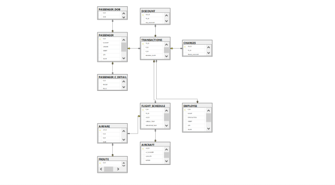
A lot of manuals group symbols into labeled blocks that represent a subsystem. You might see a box labeled POWER DISTRIBUTION that contains fuses, relays, and main feeds — that tells you “all of this works together.” Arrows leaving that block, paired with short labels, tell you which downstream circuits get protected power inside “Microsoft Visio Class Diagram Tutorial”.

Inside those blocks, short codes are consistent and meaningful. Labels like F/PMP RELAY, COOL FAN CTRL, IGN COIL PWR, SNSR GND tell you fuel pump actuation, fan control path, ignition feed, and sensor-only ground. Colors are given as pairs (BRN/ORG, BLK/WHT) to help you follow the physical loom for “Microsoft Visio Class Diagram Tutorial”.

When you splice or extend the loom in Diagram Tutorial, keep the printed IDs the same in 2025. If you rewrite connector numbers or colors, the next failure will look like http://mydiagram.online caused it. Instead, mirror the original tags and record your work path in https://http://mydiagram.online/microsoft-visio-class-diagram-tutorial/MYDIAGRAM.ONLINE so the “Microsoft Visio Class Diagram Tutorial” system remains traceable.

Wire colors and gauges are not random choices; they are deliberate engineering decisions that ensure a circuit performs as designed.
Insulation color offers an immediate clue to the wire’s purpose, and its diameter dictates the safe current-carrying limit.
For example, in a complex control system, red wires typically deliver constant voltage, yellow wires handle ignition or switched power, and black wires connect to ground.
Disregarding color standards causes chaos in diagnostics and increases risk when more than one technician works on “Microsoft Visio Class Diagram Tutorial”.
Consistency in color and gauge coding improves safety and keeps maintenance records traceable in “Microsoft Visio Class Diagram Tutorial”.

In Diagram Tutorial, wiring standards are shaped by decades of international collaboration between automotive, industrial, and electronics sectors.
Standards such as ISO 6722, SAE J1128, and IEC 60228 describe conductor materials, size ranges, and temperature limits.
They also cover insulation, marking, and current-testing requirements to ensure reliability.
A 2.5 mm² or 14 AWG cable usually supports 25A at room temperature, yet needs derating in hotter climates.
Applying these standards avoids overheating, power loss, and system failure, guaranteeing reliability for “Microsoft Visio Class Diagram Tutorial”.

Technicians must record all wiring changes carefully to maintain traceability.
When replacing or adding cables, always match the original wire color and gauge as closely as possible.
If substitution is required, verify ampacity and insulation quality before use.
Color tags or printed sleeves preserve consistency when temporary or alternate cables are used.
Once finished, record updates in http://mydiagram.online, include the date (2025), and store revised diagrams at https://http://mydiagram.online/microsoft-visio-class-diagram-tutorial/MYDIAGRAM.ONLINE.
This documentation habit protects both the technician and the organization by creating a transparent service history for future diagnostics.

Power distribution is essential to maintaining safe, stable, and efficient electrical performance.
It manages the controlled division of energy from a main source into multiple circuits powering “Microsoft Visio Class Diagram Tutorial”.
A proper power network keeps voltage steady, prevents overloads, and safeguards delicate devices.
Without proper power management, circuits may experience instability, equipment failure, or even safety hazards.
Proper design guarantees that all circuits run smoothly and safely under any operating condition.

The process of building an efficient power distribution network starts with understanding total power demand.
Wires, relays, and protection devices must be chosen according to load, temperature, and conditions.
In Diagram Tutorial, engineers typically refer to ISO 16750, IEC 61000, and SAE J1113 to ensure design consistency and compliance.
Cables carrying high current should be separated from communication or control lines to prevent signal distortion.
Relay and fuse locations should be arranged for convenience and quick inspection.
Following these design rules helps “Microsoft Visio Class Diagram Tutorial” operate efficiently and stay immune to electrical disturbances.

After installation, every power distribution system must undergo testing and validation.
Inspectors must test voltage, continuity, and insulation strength to ensure the network functions correctly.
Revisions and wiring updates must appear in both drawings and digital records.
Inspection reports, voltage measurements, and photos should be stored securely in http://mydiagram.online for long-term reference.
Adding the project year (2025) and reference link (https://http://mydiagram.online/microsoft-visio-class-diagram-tutorial/MYDIAGRAM.ONLINE) creates a clear, traceable documentation trail.
Comprehensive validation and logging ensure “Microsoft Visio Class Diagram Tutorial” stays dependable, compliant, and operational.

Grounding forms the essential base of electrical protection, ensuring reliability and fault prevention.
It provides a deliberate, low-resistance pathway for electrical current to flow safely into the earth during abnormal conditions.
Without grounding, “Microsoft Visio Class Diagram Tutorial” may be exposed to dangerous voltages, unpredictable surges, and potential equipment failure.
An effective grounding network ensures steady current, improved safety, and reduced system failure.
Within Diagram Tutorial, grounding has become an enforced standard for all certified electrical systems.

Building a reliable grounding layout begins with analyzing soil resistance, moisture, and site design.
Connections must be mechanically tight, corrosion-free, and dimensioned for full current handling.
Within Diagram Tutorial, grounding designs adhere to IEC 60364 and IEEE 142 for international safety compliance.
Electrodes should be installed deep enough to ensure stable resistance under varying soil conditions.
All grounding points and metallic parts should be interconnected to maintain equal potential throughout the system.
Following these standards allows “Microsoft Visio Class Diagram Tutorial” to operate reliably and meet electrical safety codes.

Routine verification and maintenance are key to preserving grounding effectiveness and safety.
Technicians must measure resistance levels, verify bonding continuity, and record data for future analysis.
If any anomaly or corrosion is detected, immediate maintenance and retesting should be performed.
Maintenance logs and test results must be preserved to meet safety audit requirements.
Testing should occur every 2025 or after significant changes in the installation environment.
Continuous inspection and documentation help “Microsoft Visio Class Diagram Tutorial” preserve safety, reliability, and performance.

Microsoft Visio Class Diagram Tutorial – Connector Index & Pinout Guide 2025

Every wiring diagram specifies connector orientation to maintain accurate circuit layout. {Most service manuals indicate whether the connector is viewed from the terminal side or the wire side.|Diagrams are labeled “view from harness side” or “view from pin side” for clarity.|Orientation notes are mandatory i...

If the view direction is misunderstood, testing or wiring could be done on the wrong terminals. Cross-checking connector photos and diagrams prevents costly diagnostic mistakes.

Markings on the connector body assist in verifying correct terminal orientation. {Maintaining orientation accuracy ensures safe wiring repair and consistent performance across systems.|Correct connector alignment guarantees reliable current flow and long-term harness durability.|Following orientation standards protects agains...

Microsoft Visio Class Diagram Tutorial Full Manual – Sensor Inputs Reference 2025

The Accelerator Pedal Position (APP) sensor detects how far the accelerator pedal is pressed. {It replaces traditional throttle cables with electronic signals that connect the pedal to the throttle body.|By eliminating mechanical linkage, APP systems improve response and reduce maintenance.|Electronic throttle control (ET...

Most APP sensors use dual potentiometers for redundancy and safety. Each sensor circuit provides a proportional signal representing pedal travel.

Technicians should monitor live data and verify signal correlation between channels. {Maintaining APP sensor integrity ensures smooth throttle response and safe vehicle operation.|Proper calibration and diagnostics improve system reliability and drivability.|Understanding APP signal processing helps technicians fine-tune performance an...

Microsoft Visio Class Diagram Tutorial Full Manual – Actuator Outputs Guide 2025

Each solenoid opens or closes fluid passages to engage specific clutches or bands. {Transmission control units (TCUs) send pulse-width modulation signals to regulate pressure and timing.|Precise solenoid control ensures efficient gear changes and reduced wear.|Electronic shift solenoids have replaced older mechanic...

There are several types of transmission solenoids including shift, pressure control, and lock-up solenoids. {Each solenoid operates with a 12V power feed and is grounded through the control module transistor.|The control pulse frequency determines how much hydraulic pressure is applied.|Temperature and load data are...

Common transmission solenoid issues include sticking valves, open circuits, or internal leakage. {Proper maintenance of transmission actuators ensures smoother gear changes and longer gearbox life.|Understanding solenoid output control helps pinpoint hydraulic and electrical faults.|Correct diagnosis prevents major transmission dama...

Microsoft Visio Class Diagram Tutorial Full Manual – Actuator Outputs Reference 2025

Each solenoid opens or closes fluid passages to engage specific clutches or bands. {Transmission control units (TCUs) send pulse-width modulation signals to regulate pressure and timing.|Precise solenoid control ensures efficient gear changes and reduced wear.|Electronic shift solenoids have replaced older mechanic...

There are several types of transmission solenoids including shift, pressure control, and lock-up solenoids. {Each solenoid operates with a 12V power feed and is grounded through the control module transistor.|The control pulse frequency determines how much hydraulic pressure is applied.|Temperature and load data are...

Technicians should check resistance values and use scan tools to monitor duty cycle operation. {Proper maintenance of transmission actuators ensures smoother gear changes and longer gearbox life.|Understanding solenoid output control helps pinpoint hydraulic and electrical faults.|Correct diagnosis prevents major transmission dama...

As the distributed nervous system of the
vehicle, the communication bus eliminates bulky point-to-point wiring by
delivering unified message pathways that significantly reduce harness
mass and electrical noise. By enforcing timing discipline and
arbitration rules, the system ensures each module receives critical
updates without interruption.

High-speed CAN governs engine timing, ABS
logic, traction strategies, and other subsystems that require real-time
message exchange, while LIN handles switches and comfort electronics.
FlexRay supports chassis-level precision, and Ethernet transports camera
and radar data with minimal latency.

Technicians often
identify root causes such as thermal cycling, micro-fractured
conductors, or grounding imbalances that disrupt stable signaling.
Careful inspection of routing, shielding continuity, and connector
integrity restores communication reliability.

Protection systems in Microsoft Visio Class Diagram Tutorial 2025 Diagram Tutorial rely on fuses and relays
to form a controlled barrier between electrical loads and the vehicle’s
power distribution backbone. These elements react instantly to abnormal
current patterns, stopping excessive amperage before it cascades into
critical modules. By segmenting circuits into isolated branches, the
system protects sensors, control units, lighting, and auxiliary
equipment from thermal stress and wiring burnout.

In modern architectures, relays handle repetitive activation
cycles, executing commands triggered by sensors or control software.
Their isolation capabilities reduce stress on low‑current circuits,
while fuses provide sacrificial protection whenever load spikes exceed
tolerance thresholds. Together they create a multi‑layer defense grid
adaptable to varying thermal and voltage demands.

Common failures within fuse‑relay assemblies often trace back to
vibration fatigue, corroded terminals, oxidized blades, weak coil
windings, or overheating caused by loose socket contacts. Drivers may
observe symptoms such as flickering accessories, intermittent actuator
response, disabled subsystems, or repeated fuse blows. Proper
diagnostics require voltage‑drop measurements, socket stability checks,
thermal inspection, and coil resistance evaluation.

Within modern automotive systems,
reference pads act as structured anchor locations for communication
frame irregularities, enabling repeatable and consistent measurement
sessions. Their placement across sensor returns, control-module feeds,
and distribution junctions ensures that technicians can evaluate
baseline conditions without interference from adjacent circuits. This
allows diagnostic tools to interpret subsystem health with greater
accuracy.

Using their strategic layout, test points enable
communication frame irregularities, ensuring that faults related to
thermal drift, intermittent grounding, connector looseness, or voltage
instability are detected with precision. These checkpoints streamline
the troubleshooting workflow by eliminating unnecessary inspection of
unrelated harness branches and focusing attention on the segments most
likely to generate anomalies.

Frequent discoveries made at reference nodes
involve irregular waveform signatures, contact oxidation, fluctuating
supply levels, and mechanical fatigue around connector bodies.
Diagnostic procedures include load simulation, voltage-drop mapping, and
ground potential verification to ensure that each subsystem receives
stable and predictable electrical behavior under all operating
conditions.

In modern
systems, structured diagnostics rely heavily on duty-cycle pattern
validation, allowing technicians to capture consistent reference data
while minimizing interference from adjacent circuits. This structured
approach improves accuracy when identifying early deviations or subtle
electrical irregularities within distributed subsystems.

Technicians utilize these measurements to evaluate waveform stability,
frequency-stability testing, and voltage behavior across multiple
subsystem domains. Comparing measured values against specifications
helps identify root causes such as component drift, grounding
inconsistencies, or load-induced fluctuations.

Frequent
anomalies identified during procedure-based diagnostics include ground
instability, periodic voltage collapse, digital noise interference, and
contact resistance spikes. Consistent documentation and repeated
sampling are essential to ensure accurate diagnostic conclusions.

Structured troubleshooting depends on
pre-evaluation step mapping, enabling technicians to establish reliable
starting points before performing detailed inspections.

Technicians use communication-frame timing checks to narrow fault
origins. By validating electrical integrity and observing behavior under
controlled load, they identify abnormal deviations early.

Voltage-drop asymmetry
across multi-branch distribution circuits frequently signals cumulative
connector degradation. Mapping cross-branch differentials helps locate
the failing node.

Across diverse vehicle architectures, issues related to
connector microfractures producing millisecond dropouts represent a
dominant source of unpredictable faults. These faults may develop
gradually over months of thermal cycling, vibrations, or load
variations, ultimately causing operational anomalies that mimic
unrelated failures. Effective troubleshooting requires technicians to
start with a holistic overview of subsystem behavior, forming accurate
expectations about what healthy signals should look like before
proceeding.

Patterns
linked to connector microfractures producing millisecond dropouts
frequently reveal themselves during active subsystem transitions, such
as ignition events, relay switching, or electronic module
initialization. The resulting irregularities—whether sudden voltage
dips, digital noise pulses, or inconsistent ground offset—are best
analyzed using waveform-capture tools that expose micro-level
distortions invisible to simple multimeter checks.

Left unresolved, connector microfractures
producing millisecond dropouts may cause cascading failures as modules
attempt to compensate for distorted data streams. This can trigger false
DTCs, unpredictable load behavior, delayed actuator response, and even
safety-feature interruptions. Comprehensive analysis requires reviewing
subsystem interaction maps, recreating stress conditions, and validating
each reference point’s consistency under both static and dynamic
operating states.

Maintenance and best practices for Microsoft Visio Class Diagram Tutorial 2025 Diagram Tutorial place
strong emphasis on low-current circuit preservation strategies, ensuring
that electrical reliability remains consistent across all operating
conditions. Technicians begin by examining the harness environment,
verifying routing paths, and confirming that insulation remains intact.
This foundational approach prevents intermittent issues commonly
triggered by heat, vibration, or environmental contamination.

Technicians
analyzing low-current circuit preservation strategies typically monitor
connector alignment, evaluate oxidation levels, and inspect wiring for
subtle deformations caused by prolonged thermal exposure. Protective
dielectric compounds and proper routing practices further contribute to
stable electrical pathways that resist mechanical stress and
environmental impact.

Failure
to maintain low-current circuit preservation strategies can lead to
cascading electrical inconsistencies, including voltage drops, sensor
signal distortion, and sporadic subsystem instability. Long-term
reliability requires careful documentation, periodic connector service,
and verification of each branch circuit’s mechanical and electrical
health under both static and dynamic conditions.

The appendix for Microsoft Visio Class Diagram Tutorial 2025 Diagram Tutorial serves as a consolidated
reference hub focused on subsystem classification nomenclature, offering
technicians consistent terminology and structured documentation
practices. By collecting technical descriptors, abbreviations, and
classification rules into a single section, the appendix streamlines
interpretation of wiring layouts across diverse platforms. This ensures
that even complex circuit structures remain approachable through
standardized definitions and reference cues.

Material within the appendix covering subsystem
classification nomenclature often features quick‑access charts,
terminology groupings, and definition blocks that serve as anchors
during diagnostic work. Technicians rely on these consolidated
references to differentiate between similar connector profiles,
categorize branch circuits, and verify signal classifications.

Comprehensive references for subsystem classification nomenclature also
support long‑term documentation quality by ensuring uniform terminology
across service manuals, schematics, and diagnostic tools. When updates
occur—whether due to new sensors, revised standards, or subsystem
redesigns—the appendix remains the authoritative source for maintaining
alignment between engineering documentation and real‑world service
practices.

Signal‑integrity evaluation must account for the influence of
jitter accumulation across communication cycles, as even minor waveform
displacement can compromise subsystem coordination. These variances
affect module timing, digital pulse shape, and analog accuracy,
underscoring the need for early-stage waveform sampling before deeper
EMC diagnostics.

Patterns associated with jitter accumulation across
communication cycles often appear during subsystem switching—ignition
cycles, relay activation, or sudden load redistribution. These events
inject disturbances through shared conductors, altering reference
stability and producing subtle waveform irregularities. Multi‑state
capture sequences are essential for distinguishing true EMC faults from
benign system noise.

If jitter
accumulation across communication cycles persists, cascading instability
may arise: intermittent communication, corrupt data frames, or erratic
control logic. Mitigation requires strengthening shielding layers,
rebalancing grounding networks, refining harness layout, and applying
proper termination strategies. These corrective steps restore signal
coherence under EMC stress.

Advanced EMC evaluation in Microsoft Visio Class Diagram Tutorial 2025 Diagram Tutorial requires close
study of return‑path discontinuities generating unstable references, a
phenomenon that can significantly compromise waveform predictability. As
systems scale toward higher bandwidth and greater sensitivity, minor
deviations in signal symmetry or reference alignment become amplified.
Understanding the initial conditions that trigger these distortions
allows technicians to anticipate system vulnerabilities before they
escalate.

When return‑path discontinuities generating unstable references is
present, it may introduce waveform skew, in-band noise, or pulse
deformation that impacts the accuracy of both analog and digital
subsystems. Technicians must examine behavior under load, evaluate the
impact of switching events, and compare multi-frequency responses.
High‑resolution oscilloscopes and field probes reveal distortion
patterns hidden in time-domain measurements.

If left unresolved, return‑path
discontinuities generating unstable references may trigger cascading
disruptions including frame corruption, false sensor readings, and
irregular module coordination. Effective countermeasures include
controlled grounding, noise‑filter deployment, re‑termination of
critical paths, and restructuring of cable routing to minimize
electromagnetic coupling.

Deep diagnostic exploration of signal integrity in Microsoft Visio Class Diagram Tutorial 2025
Diagram Tutorial must consider how alternator ripple noise modulating digital
communication frames alters the electrical behavior of communication
pathways. As signal frequencies increase or environmental
electromagnetic conditions intensify, waveform precision becomes
sensitive to even minor impedance gradients. Technicians therefore begin
evaluation by mapping signal propagation under controlled conditions and
identifying baseline distortion characteristics.

Systems experiencing alternator ripple noise modulating
digital communication frames often show dynamic fluctuations during
transitions such as relay switching, injector activation, or alternator
charging ramps. These transitions inject complex disturbances into
shared wiring paths, making it essential to perform frequency-domain
inspection, spectral decomposition, and transient-load waveform sampling
to fully characterize the EMC interaction.

Prolonged exposure to alternator ripple noise modulating digital
communication frames may result in cumulative timing drift, erratic
communication retries, or persistent sensor inconsistencies. Mitigation
strategies include rebalancing harness impedance, reinforcing shielding
layers, deploying targeted EMI filters, optimizing grounding topology,
and refining cable routing to minimize exposure to EMC hotspots. These
measures restore signal clarity and long-term subsystem reliability.

Deep technical assessment of signal behavior in Microsoft Visio Class Diagram Tutorial 2025
Diagram Tutorial requires understanding how burst-noise propagation triggered by
module wake‑sequence surges reshapes waveform integrity across
interconnected circuits. As system frequency demands rise and wiring
architectures grow more complex, even subtle electromagnetic
disturbances can compromise deterministic module coordination. Initial
investigation begins with controlled waveform sampling and baseline
mapping.

When burst-noise propagation triggered by module wake‑sequence surges
is active, waveform distortion may manifest through amplitude
instability, reference drift, unexpected ringing artifacts, or shifting
propagation delays. These effects often correlate with subsystem
transitions, thermal cycles, actuator bursts, or environmental EMI
fluctuations. High‑bandwidth test equipment reveals the microscopic
deviations hidden within normal signal envelopes.

If unresolved, burst-noise propagation
triggered by module wake‑sequence surges may escalate into severe
operational instability, corrupting digital frames or disrupting
tight‑timing control loops. Effective mitigation requires targeted
filtering, optimized termination schemes, strategic rerouting, and
harmonic suppression tailored to the affected frequency bands.

In-depth
signal integrity analysis requires understanding how lossy‑media
propagation degrading analog sensor fidelity influences propagation
across mixed-frequency network paths. These distortions may remain
hidden during low-load conditions, only becoming evident when multiple
modules operate simultaneously or when thermal boundaries shift.

When lossy‑media propagation degrading analog sensor fidelity is
active, signal paths may exhibit ringing artifacts, asymmetric edge
transitions, timing drift, or unexpected amplitude compression. These
effects are amplified during actuator bursts, ignition sequencing, or
simultaneous communication surges. Technicians rely on high-bandwidth
oscilloscopes and spectral analysis to characterize these distortions
accurately.

Long-term exposure to lossy‑media propagation degrading analog sensor
fidelity can lead to cumulative communication degradation, sporadic
module resets, arbitration errors, and inconsistent sensor behavior.
Technicians mitigate these issues through grounding rebalancing,
shielding reinforcement, optimized routing, precision termination, and
strategic filtering tailored to affected frequency bands.

Advanced EMC analysis in Microsoft Visio Class Diagram Tutorial 2025 Diagram Tutorial must consider
electric-motor commutation noise saturating analog sensor thresholds, a
complex interaction capable of reshaping waveform integrity across
numerous interconnected subsystems. As modern vehicles integrate
high-speed communication layers, ADAS modules, EV power electronics, and
dense mixed-signal harness routing, even subtle non-linear effects can
disrupt deterministic timing and system reliability.

Systems experiencing electric-motor commutation noise
saturating analog sensor thresholds frequently display instability
during high-demand or multi-domain activity. These effects stem from
mixed-frequency coupling, high-voltage switching noise, radiated
emissions, or environmental field density. Analyzing time-domain and
frequency-domain behavior together is essential for accurate root-cause
isolation.

Long-term exposure to electric-motor commutation noise saturating
analog sensor thresholds may degrade subsystem coherence, trigger
inconsistent module responses, corrupt data frames, or produce rare but
severe system anomalies. Mitigation strategies include optimized
shielding architecture, targeted filter deployment, rerouting vulnerable
harness paths, reinforcing isolation barriers, and ensuring ground
uniformity throughout critical return networks.

In-depth planning of
harness architecture involves understanding how strain‑relief
architecture preventing micro‑fractures in tight bends affects long-term
stability. As wiring systems grow more complex, engineers must consider
structural constraints, subsystem interaction, and the balance between
electrical separation and mechanical compactness.

During layout development, strain‑relief architecture preventing
micro‑fractures in tight bends can determine whether circuits maintain
clean signal behavior under dynamic operating conditions. Mechanical and
electrical domains intersect heavily in modern harness designs—routing
angle, bundling tightness, grounding alignment, and mounting intervals
all affect susceptibility to noise, wear, and heat.

Proper control of strain‑relief architecture preventing micro‑fractures
in tight bends ensures reliable operation, simplified manufacturing, and
long-term durability. Technicians and engineers apply routing
guidelines, shielding rules, and structural anchoring principles to
ensure consistent performance regardless of environment or subsystem
load.

The engineering process behind
Harness Layout Variant #2 evaluates how dynamic routing paths adapted
for moving chassis components interacts with subsystem density, mounting
geometry, EMI exposure, and serviceability. This foundational planning
ensures clean routing paths and consistent system behavior over the
vehicle’s full operating life.

During refinement, dynamic routing paths adapted for moving chassis
components impacts EMI susceptibility, heat distribution, vibration
loading, and ground continuity. Designers analyze spacing, elevation
changes, shielding alignment, tie-point positioning, and path curvature
to ensure the harness resists mechanical fatigue while maintaining
electrical integrity.

If neglected,
dynamic routing paths adapted for moving chassis components may cause
abrasion, insulation damage, intermittent electrical noise, or alignment
stress on connectors. Precision anchoring, balanced tensioning, and
correct separation distances significantly reduce such failure risks
across the vehicle’s entire electrical architecture.

Harness Layout Variant #3 for Microsoft Visio Class Diagram Tutorial 2025 Diagram Tutorial focuses on
water‑diversion routing strategies for lower chassis layouts, an
essential structural and functional element that affects reliability
across multiple vehicle zones. Modern platforms require routing that
accommodates mechanical constraints while sustaining consistent
electrical behavior and long-term durability.

In real-world operation, water‑diversion
routing strategies for lower chassis layouts determines how the harness
responds to thermal cycling, chassis motion, subsystem vibration, and
environmental elements. Proper connector staging, strategic bundling,
and controlled curvature help maintain stable performance even in
aggressive duty cycles.

If not addressed,
water‑diversion routing strategies for lower chassis layouts may lead to
premature insulation wear, abrasion hotspots, intermittent electrical
noise, or connector fatigue. Balanced tensioning, routing symmetry, and
strategic material selection significantly mitigate these risks across
all major vehicle subsystems.

The
architectural approach for this variant prioritizes anti-abrasion sleeve strategies for sharp-edge pass-
throughs, focusing on service access, electrical noise reduction, and long-term durability. Engineers balance
bundle compactness with proper signal separation to avoid EMI coupling while keeping the routing footprint
efficient.

In real-world operation, anti-abrasion sleeve strategies for sharp-edge pass-throughs
affects signal quality near actuators, motors, and infotainment modules. Cable elevation, branch sequencing,
and anti-chafe barriers reduce premature wear. A combination of elastic tie-points, protective sleeves, and
low-profile clips keeps bundles orderly yet flexible under dynamic loads.

Proper control of anti-abrasion
sleeve strategies for sharp-edge pass-throughs minimizes moisture intrusion, terminal corrosion, and cross-
path noise. Best practices include labeled manufacturing references, measured service loops, and HV/LV
clearance audits. When components are updated, route documentation and measurement points simplify
verification without dismantling the entire assembly.

The initial stage of
Diagnostic Flowchart #1 emphasizes dynamic load simulation to reproduce transient bus failures, ensuring that
the most foundational electrical references are validated before branching into deeper subsystem evaluation.
This reduces misdirection caused by surface‑level symptoms. Mid‑stage analysis integrates dynamic load
simulation to reproduce transient bus failures into a structured decision tree, allowing each measurement to
eliminate specific classes of faults. By progressively narrowing the fault domain, the technician accelerates
isolation of underlying issues such as inconsistent module timing, weak grounds, or intermittent sensor
behavior. If dynamic load simulation to reproduce transient bus failures is
not thoroughly validated, subtle faults can cascade into widespread subsystem instability. Reinforcing each
decision node with targeted measurements improves long‑term reliability and prevents misdiagnosis.

The initial phase of Diagnostic Flowchart #2 emphasizes structured
isolation of subsystem power dependencies, ensuring that technicians validate foundational electrical
relationships before evaluating deeper subsystem interactions. This prevents diagnostic drift and reduces
unnecessary component replacements. Throughout the flowchart,
structured isolation of subsystem power dependencies interacts with verification procedures involving
reference stability, module synchronization, and relay or fuse behavior. Each decision point eliminates entire
categories of possible failures, allowing the technician to converge toward root cause faster. If structured isolation of subsystem
power dependencies is not thoroughly examined, intermittent signal distortion or cascading electrical faults
may remain hidden. Reinforcing each decision node with precise measurement steps prevents misdiagnosis and
strengthens long-term reliability.

The first branch of Diagnostic Flowchart #3 prioritizes thermal‑dependent CAN dropout
reproduction, ensuring foundational stability is confirmed before deeper subsystem exploration. This prevents
misdirection caused by intermittent or misleading electrical behavior. Throughout the analysis, thermal‑dependent CAN dropout
reproduction interacts with branching decision logic tied to grounding stability, module synchronization, and
sensor referencing. Each step narrows the diagnostic window, improving root‑cause accuracy. If thermal‑dependent CAN dropout reproduction is not thoroughly
verified, hidden electrical inconsistencies may trigger cascading subsystem faults. A reinforced decision‑tree
process ensures all potential contributors are validated.

Diagnostic Flowchart #4 for Microsoft Visio Class Diagram Tutorial 2025
Diagram Tutorial focuses on hybrid HV/LV interference tracking using flow branches, laying the foundation for a
structured fault‑isolation path that eliminates guesswork and reduces unnecessary component swapping. The
first stage examines core references, voltage stability, and baseline communication health to determine
whether the issue originates in the primary network layer or in a secondary subsystem. Technicians follow a
branched decision flow that evaluates signal symmetry, grounding patterns, and frame stability before
advancing into deeper diagnostic layers. As the evaluation continues, hybrid HV/LV interference tracking
using flow branches becomes the controlling factor for mid‑level branch decisions. This includes correlating
waveform alignment, identifying momentary desync signatures, and interpreting module wake‑timing conflicts. By
dividing the diagnostic pathway into focused electrical domains—power delivery, grounding integrity,
communication architecture, and actuator response—the flowchart ensures that each stage removes entire
categories of faults with minimal overlap. This structured segmentation accelerates troubleshooting and
increases diagnostic precision. The final stage ensures that hybrid HV/LV interference tracking using flow branches is validated
under multiple operating conditions, including thermal stress, load spikes, vibration, and state transitions.
These controlled stress points help reveal hidden instabilities that may not appear during static testing.
Completing all verification nodes ensures long‑term stability, reducing the likelihood of recurring issues and
enabling technicians to document clear, repeatable steps for future diagnostics.

Case Study #1 for Microsoft Visio Class Diagram Tutorial 2025 Diagram Tutorial examines a real‑world failure involving instrument‑cluster data
loss from intermittent low‑voltage supply. The issue first appeared as an intermittent symptom that did not
trigger a consistent fault code, causing technicians to suspect unrelated components. Early observations
highlighted irregular electrical behavior, such as momentary signal distortion, delayed module responses, or
fluctuating reference values. These symptoms tended to surface under specific thermal, vibration, or load
conditions, making replication difficult during static diagnostic tests. Further investigation into
instrument‑cluster data loss from intermittent low‑voltage supply required systematic measurement across power
distribution paths, grounding nodes, and communication channels. Technicians used targeted diagnostic
flowcharts to isolate variables such as voltage drop, EMI exposure, timing skew, and subsystem
desynchronization. By reproducing the fault under controlled conditions—applying heat, inducing vibration, or
simulating high load—they identified the precise moment the failure manifested. This structured process
eliminated multiple potential contributors, narrowing the fault domain to a specific harness segment,
component group, or module logic pathway. The confirmed cause tied to instrument‑cluster data loss from
intermittent low‑voltage supply allowed technicians to implement the correct repair, whether through component
replacement, harness restoration, recalibration, or module reprogramming. After corrective action, the system
was subjected to repeated verification cycles to ensure long‑term stability under all operating conditions.
Documenting the failure pattern and diagnostic sequence provided valuable reference material for similar
future cases, reducing diagnostic time and preventing unnecessary part replacement.

Case Study #2 for Microsoft Visio Class Diagram Tutorial 2025 Diagram Tutorial examines a real‑world failure involving sensor contamination
leading to non‑linear analog output distortion. The issue presented itself with intermittent symptoms that
varied depending on temperature, load, or vehicle motion. Technicians initially observed irregular system
responses, inconsistent sensor readings, or sporadic communication drops. Because the symptoms did not follow
a predictable pattern, early attempts at replication were unsuccessful, leading to misleading assumptions
about unrelated subsystems. A detailed investigation into sensor contamination leading to non‑linear analog
output distortion required structured diagnostic branching that isolated power delivery, ground stability,
communication timing, and sensor integrity. Using controlled diagnostic tools, technicians applied thermal
load, vibration, and staged electrical demand to recreate the failure in a measurable environment. Progressive
elimination of subsystem groups—ECUs, harness segments, reference points, and actuator pathways—helped reveal
how the failure manifested only under specific operating thresholds. This systematic breakdown prevented
misdiagnosis and reduced unnecessary component swaps. Once the cause linked to sensor contamination leading
to non‑linear analog output distortion was confirmed, the corrective action involved either reconditioning the
harness, replacing the affected component, reprogramming module firmware, or adjusting calibration parameters.
Post‑repair validation cycles were performed under varied conditions to ensure long‑term reliability and
prevent future recurrence. Documentation of the failure characteristics, diagnostic sequence, and final
resolution now serves as a reference for addressing similar complex faults more efficiently.

Case Study #3 for Microsoft Visio Class Diagram Tutorial 2025 Diagram Tutorial focuses on a real‑world failure involving harness shielding
collapse resulting in broadband EMI intrusion. Technicians first observed erratic system behavior, including
fluctuating sensor values, delayed control responses, and sporadic communication warnings. These symptoms
appeared inconsistently, often only under specific temperature, load, or vibration conditions. Early
troubleshooting attempts failed to replicate the issue reliably, creating the impression of multiple unrelated
subsystem faults rather than a single root cause. To investigate harness shielding collapse resulting in
broadband EMI intrusion, a structured diagnostic approach was essential. Technicians conducted staged power
and ground validation, followed by controlled stress testing that included thermal loading, vibration
simulation, and alternating electrical demand. This method helped reveal the precise operational threshold at
which the failure manifested. By isolating system domains—communication networks, power rails, grounding
nodes, and actuator pathways—the diagnostic team progressively eliminated misleading symptoms and narrowed the
problem to a specific failure mechanism. After identifying the underlying cause tied to harness shielding
collapse resulting in broadband EMI intrusion, technicians carried out targeted corrective actions such as
replacing compromised components, restoring harness integrity, updating ECU firmware, or recalibrating
affected subsystems. Post‑repair validation cycles confirmed stable performance across all operating
conditions. The documented diagnostic path and resolution now serve as a repeatable reference for addressing
similar failures with greater speed and accuracy.

Case Study #4 for Microsoft Visio Class Diagram Tutorial 2025 Diagram Tutorial examines a high‑complexity real‑world failure involving sensor
resolution collapse during high‑frequency vibration exposure. The issue manifested across multiple subsystems
simultaneously, creating an array of misleading symptoms ranging from inconsistent module responses to
distorted sensor feedback and intermittent communication warnings. Initial diagnostics were inconclusive due
to the fault’s dependency on vibration, thermal shifts, or rapid load changes. These fluctuating conditions
allowed the failure to remain dormant during static testing, pushing technicians to explore deeper system
interactions that extended beyond conventional troubleshooting frameworks. To investigate sensor resolution
collapse during high‑frequency vibration exposure, technicians implemented a layered diagnostic workflow
combining power‑rail monitoring, ground‑path validation, EMI tracing, and logic‑layer analysis. Stress tests
were applied in controlled sequences to recreate the precise environment in which the instability
surfaced—often requiring synchronized heat, vibration, and electrical load modulation. By isolating
communication domains, verifying timing thresholds, and comparing analog sensor behavior under dynamic
conditions, the diagnostic team uncovered subtle inconsistencies that pointed toward deeper system‑level
interactions rather than isolated component faults. After confirming the root mechanism tied to sensor
resolution collapse during high‑frequency vibration exposure, corrective action involved component
replacement, harness reconditioning, ground‑plane reinforcement, or ECU firmware restructuring depending on
the failure’s nature. Technicians performed post‑repair endurance tests that included repeated thermal
cycling, vibration exposure, and electrical stress to guarantee long‑term system stability. Thorough
documentation of the analysis method, failure pattern, and final resolution now serves as a highly valuable
reference for identifying and mitigating similar high‑complexity failures in the future.

Case Study #5 for Microsoft Visio Class Diagram Tutorial 2025 Diagram Tutorial investigates a complex real‑world failure involving alternator
ripple spread destabilizing module reference voltages. The issue initially presented as an inconsistent
mixture of delayed system reactions, irregular sensor values, and sporadic communication disruptions. These
events tended to appear under dynamic operational conditions—such as elevated temperatures, sudden load
transitions, or mechanical vibration—which made early replication attempts unreliable. Technicians encountered
symptoms occurring across multiple modules simultaneously, suggesting a deeper systemic interaction rather
than a single isolated component failure. During the investigation of alternator ripple spread destabilizing
module reference voltages, a multi‑layered diagnostic workflow was deployed. Technicians performed sequential
power‑rail mapping, ground‑plane verification, and high‑frequency noise tracing to detect hidden
instabilities. Controlled stress testing—including targeted heat application, induced vibration, and variable
load modulation—was carried out to reproduce the failure consistently. The team methodically isolated
subsystem domains such as communication networks, analog sensor paths, actuator control logic, and module
synchronization timing. This progressive elimination approach identified critical operational thresholds where
the failure reliably emerged. After determining the underlying mechanism tied to alternator ripple spread
destabilizing module reference voltages, technicians carried out corrective actions that ranged from harness
reconditioning and connector reinforcement to firmware restructuring and recalibration of affected modules.
Post‑repair validation involved repeated cycles of vibration, thermal stress, and voltage fluctuation to
ensure long‑term stability and eliminate the possibility of recurrence. The documented resolution pathway now
serves as an advanced reference model for diagnosing similarly complex failures across modern vehicle
platforms.

Case Study #6 for Microsoft Visio Class Diagram Tutorial 2025 Diagram Tutorial examines a complex real‑world failure involving ECU logic deadlock
initiated by ripple‑induced reference collapse. Symptoms emerged irregularly, with clustered faults appearing
across unrelated modules, giving the impression of multiple simultaneous subsystem failures. These
irregularities depended strongly on vibration, temperature shifts, or abrupt electrical load changes, making
the issue difficult to reproduce during initial diagnostic attempts. Technicians noted inconsistent sensor
feedback, communication delays, and momentary power‑rail fluctuations that persisted without generating
definitive fault codes. The investigation into ECU logic deadlock initiated by ripple‑induced reference
collapse required a multi‑layer diagnostic strategy combining signal‑path tracing, ground stability
assessment, and high‑frequency noise evaluation. Technicians executed controlled stress tests—including
thermal cycling, vibration induction, and staged electrical loading—to reveal the exact thresholds at which
the fault manifested. Using structured elimination across harness segments, module clusters, and reference
nodes, they isolated subtle timing deviations, analog distortions, or communication desynchronization that
pointed toward a deeper systemic failure mechanism rather than isolated component malfunction. Once ECU logic
deadlock initiated by ripple‑induced reference collapse was identified as the root failure mechanism, targeted
corrective measures were implemented. These included harness reinforcement, connector replacement, firmware
restructuring, recalibration of key modules, or ground‑path reconfiguration depending on the nature of the
instability. Post‑repair endurance runs with repeated vibration, heat cycles, and voltage stress ensured
long‑term reliability. Documentation of the diagnostic sequence and recovery pathway now provides a vital
reference for detecting and resolving similarly complex failures more efficiently in future service
operations.

Hands‑On Lab #1 for Microsoft Visio Class Diagram Tutorial 2025 Diagram Tutorial focuses on noise‑floor measurement for analog sensor lines
exposed to EMI. This exercise teaches technicians how to perform structured diagnostic measurements using
multimeters, oscilloscopes, current probes, and differential tools. The initial phase emphasizes establishing
a stable baseline by checking reference voltages, verifying continuity, and confirming ground integrity. These
foundational steps ensure that subsequent measurements reflect true system behavior rather than secondary
anomalies introduced by poor probing technique or unstable electrical conditions. During the measurement
routine for noise‑floor measurement for analog sensor lines exposed to EMI, technicians analyze dynamic
behavior by applying controlled load, capturing waveform transitions, and monitoring subsystem responses. This
includes observing timing shifts, duty‑cycle changes, ripple patterns, or communication irregularities. By
replicating real operating conditions—thermal changes, vibration, or electrical demand spikes—technicians gain
insight into how the system behaves under stress. This approach allows deeper interpretation of patterns that
static readings cannot reveal. After completing the procedure for noise‑floor measurement for analog sensor
lines exposed to EMI, results are documented with precise measurement values, waveform captures, and
interpretation notes. Technicians compare the observed data with known good references to determine whether
performance falls within acceptable thresholds. The collected information not only confirms system health but
also builds long‑term diagnostic proficiency by helping technicians recognize early indicators of failure and
understand how small variations can evolve into larger issues.

Hands‑On Lab #2 for Microsoft Visio Class Diagram Tutorial 2025 Diagram Tutorial focuses on oscilloscope‑based verification of crankshaft sensor
waveform stability. This practical exercise expands technician measurement skills by emphasizing accurate
probing technique, stable reference validation, and controlled test‑environment setup. Establishing baseline
readings—such as reference ground, regulated voltage output, and static waveform characteristics—is essential
before any dynamic testing occurs. These foundational checks prevent misinterpretation caused by poor tool
placement, floating grounds, or unstable measurement conditions. During the procedure for oscilloscope‑based
verification of crankshaft sensor waveform stability, technicians simulate operating conditions using thermal
stress, vibration input, and staged subsystem loading. Dynamic measurements reveal timing inconsistencies,
amplitude drift, duty‑cycle changes, communication irregularities, or nonlinear sensor behavior.
Oscilloscopes, current probes, and differential meters are used to capture high‑resolution waveform data,
enabling technicians to identify subtle deviations that static multimeter readings cannot detect. Emphasis is
placed on interpreting waveform shape, slope, ripple components, and synchronization accuracy across
interacting modules. After completing the measurement routine for oscilloscope‑based verification of
crankshaft sensor waveform stability, technicians document quantitative findings—including waveform captures,
voltage ranges, timing intervals, and noise signatures. The recorded results are compared to known‑good
references to determine subsystem health and detect early‑stage degradation. This structured approach not only
builds diagnostic proficiency but also enhances a technician’s ability to predict emerging faults before they
manifest as critical failures, strengthening long‑term reliability of the entire system.

Hands‑On Lab #3 for Microsoft Visio Class Diagram Tutorial 2025 Diagram Tutorial focuses on vehicle-ground potential variance tracing across body
points. This exercise trains technicians to establish accurate baseline measurements before introducing
dynamic stress. Initial steps include validating reference grounds, confirming supply‑rail stability, and
ensuring probing accuracy. These fundamentals prevent distorted readings and help ensure that waveform
captures or voltage measurements reflect true electrical behavior rather than artifacts caused by improper
setup or tool noise. During the diagnostic routine for vehicle-ground potential variance tracing across body
points, technicians apply controlled environmental adjustments such as thermal cycling, vibration, electrical
loading, and communication traffic modulation. These dynamic inputs help expose timing drift, ripple growth,
duty‑cycle deviations, analog‑signal distortion, or module synchronization errors. Oscilloscopes, clamp
meters, and differential probes are used extensively to capture transitional data that cannot be observed with
static measurements alone. After completing the measurement sequence for vehicle-ground potential variance
tracing across body points, technicians document waveform characteristics, voltage ranges, current behavior,
communication timing variations, and noise patterns. Comparison with known‑good datasets allows early
detection of performance anomalies and marginal conditions. This structured measurement methodology
strengthens diagnostic confidence and enables technicians to identify subtle degradation before it becomes a
critical operational failure.

Hands‑On Lab #4 for Microsoft Visio Class Diagram Tutorial 2025 Diagram Tutorial focuses on electronic throttle body position‑tracking accuracy
testing. This laboratory exercise builds on prior modules by emphasizing deeper measurement accuracy,
environment control, and test‑condition replication. Technicians begin by validating stable reference grounds,
confirming regulated supply integrity, and preparing measurement tools such as oscilloscopes, current probes,
and high‑bandwidth differential probes. Establishing clean baselines ensures that subsequent waveform analysis
is meaningful and not influenced by tool noise or ground drift. During the measurement procedure for
electronic throttle body position‑tracking accuracy testing, technicians introduce dynamic variations
including staged electrical loading, thermal cycling, vibration input, or communication‑bus saturation. These
conditions reveal real‑time behaviors such as timing drift, amplitude instability, duty‑cycle deviation,
ripple formation, or synchronization loss between interacting modules. High‑resolution waveform capture
enables technicians to observe subtle waveform features—slew rate, edge deformation, overshoot, undershoot,
noise bursts, and harmonic artifacts. Upon completing the assessment for electronic throttle body
position‑tracking accuracy testing, all findings are documented with waveform snapshots, quantitative
measurements, and diagnostic interpretations. Comparing collected data with verified reference signatures
helps identify early‑stage degradation, marginal component performance, and hidden instability trends. This
rigorous measurement framework strengthens diagnostic precision and ensures that technicians can detect
complex electrical issues long before they evolve into system‑wide failures.

Hands‑On Lab #5 for Microsoft Visio Class Diagram Tutorial 2025 Diagram Tutorial focuses on reference‑voltage drift analysis under EMI stress. The
session begins with establishing stable measurement baselines by validating grounding integrity, confirming
supply‑rail stability, and ensuring probe calibration. These steps prevent erroneous readings and ensure that
all waveform captures accurately reflect subsystem behavior. High‑accuracy tools such as oscilloscopes, clamp
meters, and differential probes are prepared to avoid ground‑loop artifacts or measurement noise. During the
procedure for reference‑voltage drift analysis under EMI stress, technicians introduce dynamic test conditions
such as controlled load spikes, thermal cycling, vibration, and communication saturation. These deliberate
stresses expose real‑time effects like timing jitter, duty‑cycle deformation, signal‑edge distortion, ripple
growth, and cross‑module synchronization drift. High‑resolution waveform captures allow technicians to
identify anomalies that static tests cannot reveal, such as harmonic noise, high‑frequency interference, or
momentary dropouts in communication signals. After completing all measurements for reference‑voltage drift
analysis under EMI stress, technicians document voltage ranges, timing intervals, waveform shapes, noise
signatures, and current‑draw curves. These results are compared against known‑good references to identify
early‑stage degradation or marginal component behavior. Through this structured measurement framework,
technicians strengthen diagnostic accuracy and develop long‑term proficiency in detecting subtle trends that
could lead to future system failures.

Hands‑On Lab #6 for Microsoft Visio Class Diagram Tutorial 2025 Diagram Tutorial focuses on CAN physical‑layer distortion mapping under induced
load imbalance. This advanced laboratory module strengthens technician capability in capturing high‑accuracy
diagnostic measurements. The session begins with baseline validation of ground reference integrity, regulated
supply behavior, and probe calibration. Ensuring noise‑free, stable baselines prevents waveform distortion and
guarantees that all readings reflect genuine subsystem behavior rather than tool‑induced artifacts or
grounding errors. Technicians then apply controlled environmental modulation such as thermal shocks,
vibration exposure, staged load cycling, and communication traffic saturation. These dynamic conditions reveal
subtle faults including timing jitter, duty‑cycle deformation, amplitude fluctuation, edge‑rate distortion,
harmonic buildup, ripple amplification, and module synchronization drift. High‑bandwidth oscilloscopes,
differential probes, and current clamps are used to capture transient behaviors invisible to static multimeter
measurements. Following completion of the measurement routine for CAN physical‑layer distortion mapping under
induced load imbalance, technicians document waveform shapes, voltage windows, timing offsets, noise
signatures, and current patterns. Results are compared against validated reference datasets to detect
early‑stage degradation or marginal component behavior. By mastering this structured diagnostic framework,
technicians build long‑term proficiency and can identify complex electrical instabilities before they lead to
full system failure.

Checklist & Form #1 for Microsoft Visio Class Diagram Tutorial 2025 Diagram Tutorial focuses on module wake‑sequence confirmation form. This
verification document provides a structured method for ensuring electrical and electronic subsystems meet
required performance standards. Technicians begin by confirming baseline conditions such as stable reference
grounds, regulated voltage supplies, and proper connector engagement. Establishing these baselines prevents
false readings and ensures all subsequent measurements accurately reflect system behavior. During completion
of this form for module wake‑sequence confirmation form, technicians evaluate subsystem performance under both
static and dynamic conditions. This includes validating signal integrity, monitoring voltage or current drift,
assessing noise susceptibility, and confirming communication stability across modules. Checkpoints guide
technicians through critical inspection areas—sensor accuracy, actuator responsiveness, bus timing, harness
quality, and module synchronization—ensuring each element is validated thoroughly using industry‑standard
measurement practices. After filling out the checklist for module wake‑sequence confirmation form, all
results are documented, interpreted, and compared against known‑good reference values. This structured
documentation supports long‑term reliability tracking, facilitates early detection of emerging issues, and
strengthens overall system quality. The completed form becomes part of the quality‑assurance record, ensuring
compliance with technical standards and providing traceability for future diagnostics.

Checklist & Form #2 for Microsoft Visio Class Diagram Tutorial 2025 Diagram Tutorial focuses on module initialization/wake‑sequence verification
form. This structured verification tool guides technicians through a comprehensive evaluation of electrical
system readiness. The process begins by validating baseline electrical conditions such as stable ground
references, regulated supply integrity, and secure connector engagement. Establishing these fundamentals
ensures that all subsequent diagnostic readings reflect true subsystem behavior rather than interference from
setup or tooling issues. While completing this form for module initialization/wake‑sequence verification
form, technicians examine subsystem performance across both static and dynamic conditions. Evaluation tasks
include verifying signal consistency, assessing noise susceptibility, monitoring thermal drift effects,
checking communication timing accuracy, and confirming actuator responsiveness. Each checkpoint guides the
technician through critical areas that contribute to overall system reliability, helping ensure that
performance remains within specification even during operational stress. After documenting all required
fields for module initialization/wake‑sequence verification form, technicians interpret recorded measurements
and compare them against validated reference datasets. This documentation provides traceability, supports
early detection of marginal conditions, and strengthens long‑term quality control. The completed checklist
forms part of the official audit trail and contributes directly to maintaining electrical‑system reliability
across the vehicle platform.

Checklist & Form #3 for Microsoft Visio Class Diagram Tutorial 2025 Diagram Tutorial covers sensor offset‑drift monitoring record. This
verification document ensures that every subsystem meets electrical and operational requirements before final
approval. Technicians begin by validating fundamental conditions such as regulated supply voltage, stable
ground references, and secure connector seating. These baseline checks eliminate misleading readings and
ensure that all subsequent measurements represent true subsystem behavior without tool‑induced artifacts.
While completing this form for sensor offset‑drift monitoring record, technicians review subsystem behavior
under multiple operating conditions. This includes monitoring thermal drift, verifying signal‑integrity
consistency, checking module synchronization, assessing noise susceptibility, and confirming actuator
responsiveness. Structured checkpoints guide technicians through critical categories such as communication
timing, harness integrity, analog‑signal quality, and digital logic performance to ensure comprehensive
verification. After documenting all required values for sensor offset‑drift monitoring record, technicians
compare collected data with validated reference datasets. This ensures compliance with design tolerances and
facilitates early detection of marginal or unstable behavior. The completed form becomes part of the permanent
quality‑assurance record, supporting traceability, long‑term reliability monitoring, and efficient future
diagnostics.

Checklist & Form #4 for Microsoft Visio Class Diagram Tutorial 2025 Diagram Tutorial documents ECU supply‑rail quality and ripple‑tolerance
assessment. This final‑stage verification tool ensures that all electrical subsystems meet operational,
structural, and diagnostic requirements prior to release. Technicians begin by confirming essential baseline
conditions such as reference‑ground accuracy, stabilized supply rails, connector engagement integrity, and
sensor readiness. Proper baseline validation eliminates misleading measurements and guarantees that subsequent
inspection results reflect authentic subsystem behavior. While completing this verification form for ECU
supply‑rail quality and ripple‑tolerance assessment, technicians evaluate subsystem stability under controlled
stress conditions. This includes monitoring thermal drift, confirming actuator consistency, validating signal
integrity, assessing network‑timing alignment, verifying resistance and continuity thresholds, and checking
noise immunity levels across sensitive analog and digital pathways. Each checklist point is structured to
guide the technician through areas that directly influence long‑term reliability and diagnostic
predictability. After completing the form for ECU supply‑rail quality and ripple‑tolerance assessment,
technicians document measurement results, compare them with approved reference profiles, and certify subsystem
compliance. This documentation provides traceability, aids in trend analysis, and ensures adherence to
quality‑assurance standards. The completed form becomes part of the permanent electrical validation record,
supporting reliable operation throughout the vehicle’s lifecycle.